Seq2Seq 문장생성

Sequence2Sequence 모델을 활용해서 문장생성을 수행하는 테스트를 해보겠습니다. 테스트 환경은 Google Colab의 GPU를 활용합니다.

Google Drive에 업로드되어 있는 text 파일을 읽기 위해서 필요한 라이브러리를 임포트합니다. 해당 파일을 실행시키면 아래와 같은 이미지가 표시됩니다.

해당 링크를 클릭하고 들어가면 코드 값이 나오는데 코드값을 복사해서 입력하면 구글 드라이브가 마운트 되고 구글 드라이브에 저장된 파일들을 사용할 수 있게됩니다.

from google.colab import drive
drive.mount('/content/gdrive')

정상적으로 마운트 되면 “Mounted at /content/gdrive”와 같은 텍스트가 표시됩니다.

마운트 작업이 끝나면 필요한 라이브러리 들을 임포트합니다. 파이토치(PyTorch)를 사용하기 때문에 학습에 필요한 라이브러리 들을 임포트하고 기타 numpy, pandas도 함께 임포트합니다.

config 파일에는 학습에 필요한 몇가지 파라메터가 정의되어 있습니다. 학습이 완료된 후 모델을 저장하고 다시 불러올 때에 config 데이터가 저장되어 있으면 학습된 모델의 정보를 확인할 수 있어 편리합니다.

import torch
import torch.nn as nn
import torch.optim as optim
import torch.nn.functional as F

import numpy as np
import pandas as pd
import os
from argparse import Namespace

from collections import Counter

config = Namespace(
    train_file='gdrive/***/book_of_genesis.txt', seq_size=7, batch_size=100...
)

이제 학습을 위한 파일을 읽어오겠습니다. 파일은 성경 “창세기 1장”을 학습 데이터로 활용합니다. 테스트 파일은 영문 버전을 활용합니다. 파일을 읽은 후에 공백으로 분리해서 배열에 담으면 아래와 같은 형태의 값을 가지게됩니다.

with open(config.train_file, 'r', encoding='utf-8') as f:
    text = f.read()
text = text.split()

['In', 'the', 'beginning,', 'God', 'created', 'the', 'heavens', 'and', 'the', 'earth.', 'The', 'earth', 'was', 'without', 'form', 'and', 'void,', 'and', 'darkness', 'was'...

이제 학습을 위해 중복 단어를 제거하고 word2index, index2word 형태의 데이터셋을 생성합니다. 이렇게 만들어진 데이텃셋을 통해서 각 문장을 어절 단위로 분리하고 각 배열의 인덱스 값을 맵핑해서 문장을 숫자 형태의 값을 가진 데이터로 변경해줍니다. 이 과정은 자연어를 이해하지 못하는 컴퓨터가 어떠한 작업을 수행할 수 있도록 수치 형태의 데이터로 변경하는 과정입니다.

word_counts = Counter(text)
sorted_vocab = sorted(word_counts, key=word_counts.get, reverse=True)
int_to_vocab = {k: w for k, w in enumerate(sorted_vocab)}
vocab_to_int = {w: k for k, w in int_to_vocab.items()}
n_vocab = len(int_to_vocab)

print('Vocabulary size', n_vocab)

int_text = [vocab_to_int[w] for w in text] # 전체 텍스트를 index로 변경

다음은 학습을 위한 데이터를 만드는 과정입니다. 이 과정이 중요합니다. 데이터는 source_word와 target_word로 분리합니다. source_word는 [‘In’, ‘the’, ‘beginning,’, ‘God’, ‘created’, ‘the’, ‘heavens’], target_word는 [ ‘the’, ‘beginning,’, ‘God’, ‘created’, ‘the’, ‘heavens’,’and’]의 형태입니다.
즉, source_word 문장 배열 다음에 target_word가 순서대로 등장한다는 것을 모델이 학습하도록 하는 과정입니다.

여기서 문장의 크기는 7로 정했습니다. 더 큰 사이즈로 학습을 진행하면 문장을 생성할 때 더 좋은 예측을 할 수 있겠으나 계산량이 많아져서 학습 시간이 많이 필요합니다. 테스트를 통해서 적정 수준에서 값을 정해보시기 바랍니다.

source_words = []
target_words = []
for i in range(len(int_text)):
    ss_idx, se_idx, ts_idx, te_idx = i, (config.seq_size+i), i+1, (config.seq_size+i)+1
    if len(int_text[ts_idx:te_idx]) >= config.seq_size:
        source_words.append(int_text[ss_idx:se_idx])
        target_words.append(int_text[ts_idx:te_idx])

아래와 같이 어떻게 값이 들어가 있는지를 확인해보기 위해서 간단히 10개의 데이터를 출력해보겠습니다.

for s,t in zip(source_words[0:10], target_words[0:10]):
  print('source {} -> target {}'.format(s,t))

source [106, 0, 107, 3, 32, 0, 16] -> target [0, 107, 3, 32, 0, 16, 1]
source [0, 107, 3, 32, 0, 16, 1] -> target [107, 3, 32, 0, 16, 1, 0]
source [107, 3, 32, 0, 16, 1, 0] -> target [3, 32, 0, 16, 1, 0, 26]
source [3, 32, 0, 16, 1, 0, 26] -> target [32, 0, 16, 1, 0, 26, 62]
source [32, 0, 16, 1, 0, 26, 62] -> target [0, 16, 1, 0, 26, 62, 12]
source [0, 16, 1, 0, 26, 62, 12] -> target [16, 1, 0, 26, 62, 12, 4]
source [16, 1, 0, 26, 62, 12, 4] -> target [1, 0, 26, 62, 12, 4, 108]
source [1, 0, 26, 62, 12, 4, 108] -> target [0, 26, 62, 12, 4, 108, 109]
source [0, 26, 62, 12, 4, 108, 109] -> target [26, 62, 12, 4, 108, 109, 1]
source [26, 62, 12, 4, 108, 109, 1] -> target [62, 12, 4, 108, 109, 1, 110]

이제 학습을 위해서 모델을 생성합니다. 모델은 Encoder와 Decoder로 구성됩니다. 이 두 모델을 사용하는 것이 Sequence2Sequece의 전형적인 구조입니다. 해당 모델에 대해서 궁금하신 점은 pytorch 공식 사이트를 참조하시기 바랍니다. 인코더와 디코더에 대한 자세한 설명은 아래의 그림으로 대신하겠습니다. GRU 대신에 LSTM을 사용해도 무방합니다.

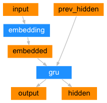
아래는 인코더의 구조입니다. 위의 그림에서와 같이 인코더는 두개의 값이 GRU 셀(Cell)로 들어가게 됩니다. 하나는 입력 값이 임베딩 레이어를 통해서 나오는 값과 또 하나는 이전 단계의 hidden 값입니다. 최종 출력은 입력을 통해서 예측된 값인 output, 다음 단계에 입력으로 들어가는 hidden이 그것입니다.

기본 구조의 seq2seq 모델에서는 output 값은 사용하지 않고 이전 단계의 hidden 값을 사용합니다. 최종 hidden 값은 입력된 문장의 전체 정보를 어떤 고정된 크기의 Context Vector에 축약하고 있기 때문에 이 값을 Decoder의 입력으로 사용합니다.

참고로 이후에 테스트할 Attention 모델은 이러한 구조와는 달리 encoder의 출력 값을 사용하는 모델입니다. 이 값을 통해서 어디에 집중할지를 정하게 됩니다.

class Encoder(nn.Module):

    def __init__(self, input_size, hidden_size):
        super().__init__()
        self.hidden_size = hidden_size
        self.embedding = nn.Embedding(input_size, hidden_size) #199->10
        self.gru = nn.GRU(hidden_size, hidden_size) #20-20

    def forward(self, x, hidden):
        x = self.embedding(x).view(1,1,-1)
        #print('Encoder forward embedding size {}'.format(x.size()))
        x, hidden = self.gru(x, hidden)
        return x, hidden

이제 아래의 그림과 같이 Decoder를 설계합니다. Decoder 역시 GRU 셀(Cell)을 가지고 있습니다.

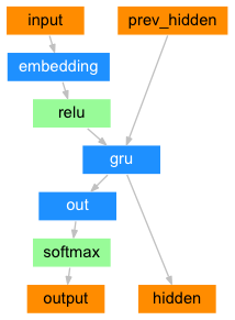
class Decoder(nn.Module):
    def __init__(self, hidden_size, output_size):
        super().__init__()
        self.hidden_size = hidden_size
        self.embedding = nn.Embedding(output_size, hidden_size) #199->10
        self.gru = nn.GRU(hidden_size, hidden_size) #10->10
        self.out = nn.Linear(hidden_size, output_size) #10->199
        self.softmax = nn.LogSoftmax(dim=1)
        
    def forward(self, x, hidden):
        x = self.embedding(x).view(1,1,-1)
        x, hidden = self.gru(x, hidden)
        x = self.softmax(self.out(x[0]))
        return x, hidden

이제 GPU를 사용하기 위해서 설정을 수행합니다. Google Colab을 활용하시면 별도의 설정작업 없이 GPU를 사용할 수 있습니다.

device = torch.device('cuda' if torch.cuda.is_available() else 'cpu')
print(device)

인코더와 디코더 입출력 정보를 셋팅합니다.

enc_hidden_size = 50
dec_hidden_size = enc_hidden_size
encoder = Encoder(n_vocab, enc_hidden_size).to(device) # source(199) -> embedding(10)
decoder = Decoder(dec_hidden_size, n_vocab).to(device) # embedding(199) -> target(199)

encoder_optimizer = optim.SGD(encoder.parameters(), lr=0.01)
decoder_optimizer = optim.SGD(decoder.parameters(), lr=0.01)

criterion = nn.NLLLoss()

해당 모델의 이미지를 아래의 그림과 같이 나타낼 수 있습니다.

Encoder(
  (embedding): Embedding(199, 50)
  (gru): GRU(50, 50)
)
Decoder(
  (embedding): Embedding(199, 50)
  (gru): GRU(50, 50)
  (out): Linear(in_features=50, out_features=199, bias=True)
  (softmax): LogSoftmax(dim=1)
)

데이터를 100개씩 나눠서 훈련 할 수 있도록 배치 모델을 작성합니다.

pairs = list(zip(source_words, target_words))
def get_batch(pairs, batch_size):
  pairs_length = len(pairs)
  for ndx in range(0, pairs_length, batch_size):
    #print(ndx, min(ndx+batch_size, pairs_length))
    yield pairs[ndx:min(ndx+batch_size, pairs_length)]

해당 모델은 500번 학습을 수행합니다. 각 batch, epoch 마다 loss 정보를 표시합니다. 표1 은 마지막 스텝의 loss와 epoch 정보입니다.

number_of_epochs = 501
for epoch in range(number_of_epochs):
    total_loss = 0
    #for pair in get_batch(pairs, config.batch_size): # batch_size 100
    for pair in get_batch(pairs, 100): # batch_size 100
      batch_loss = 0
       
      for si, ti in pair:
        x = torch.Tensor(np.array([si])).long().view(-1,1).to(device)
        y = torch.Tensor(np.array([ti])).long().view(-1,1).to(device)
        encoder_hidden = torch.zeros(1,1,enc_hidden_size).to(device)

        for j in range(config.seq_size):
            _, encoder_hidden = encoder(x[j], encoder_hidden)

        decoder_hidden = encoder_hidden
        decoder_input = torch.Tensor([[0]]).long().to(device)

        loss = 0

        for k in range(config.seq_size):
            decoder_output, decoder_hidden = decoder(decoder_input, decoder_hidden)
            decoder_input = y[k]
            loss += criterion(decoder_output, y[k])

        batch_loss += loss.item()/config.seq_size
        encoder_optimizer.zero_grad()
        decoder_optimizer.zero_grad()

        loss.backward()

        encoder_optimizer.step()
        decoder_optimizer.step()

      total_loss += batch_loss/config.batch_size
      print('batch_loss {:.5f}'.format(batch_loss/config.batch_size))
    print('epoch {}, loss {:.10f}'.format(epoch, total_loss/(len(pairs)//config.batch_size)))

...
batch_loss 0.00523
batch_loss 0.00766
batch_loss 0.01120
batch_loss 0.00735
batch_loss 0.01218
batch_loss 0.00873
batch_loss 0.00352
batch_loss 0.00377
epoch 500, loss 0.0085196330

표1. 마지막 batch, epoch 학습 정보

학습이 종료된 모델을 저장소에 저장합니다. 저장 할 때에 학습 정보가 저장되어 있는 config 내용도 포함하는 것이 좋습니다.

# Save best model weights.
torch.save({
  'encoder': encoder.state_dict(), 'decoder':decoder.state_dict(),
  'config': config,
}, 'gdrive/***/model.genesis.210122')

학습이 완료된 후에 해당 모델이 잘 학습되었는지 확인해보겠습니다. 학습은 “darkness was”라는 몇가지 단어를 주고 모델이 어떤 문장을 생성하는 지를 알아 보는 방식으로 수행합니다.

decoded_words = []

words = [vocab_to_int['darkness'], vocab_to_int['was']]
x = torch.Tensor(words).long().view(-1,1).to(device)

encoder_hidden = torch.zeros(1,1,enc_hidden_size).to(device)

for j in range(x.size(0)):
    _, encoder_hidden = encoder(x[j], encoder_hidden)

decoder_hidden = encoder_hidden
decoder_input = torch.Tensor([[words[1]]]).long().to(device)  

for di in range(20):
  decoder_output, decoder_hidden = decoder(decoder_input, decoder_hidden)
  _, top_index = decoder_output.data.topk(1)
  decoded_words.append(int_to_vocab[top_index.item()])

  decoder_input = top_index.squeeze().detach()

predict_words = decoded_words    
predict_sentence = ' '.join(predict_words)
print(predict_sentence)